“Subtraction: Addition’s Tricky Pal”
A key task in machine learning is to find data representations that are suitable for a given task. In contemporary terminology, we call this representation learning. The practical pipeline in which we learn representations as sketched out in the figure: given data, we map to some representation space in which we perform the action of interest (classification, regression, etc.)

For example, many feed-forward neural network can be viewed as extracting features to which a logistic regression classifier is applied.
In unsupervised learning things are not quite as clear cut as it isn’t particularly clear exactly what we will be doing with the learned representation. Consider an autoencoder style model, where data is mapped to a low-dimensional representation space, and then mapped back to data space with the objective of reconstructing the original data. What exactly can we do in this learned representation?
Commonly, we use this learned representation for
- Visualization: we plot the data within the new representation, and draw conclusions about the intrinsic structure of data. The hope is that new scientific insights into the behavior of the data generating phenomena can be found through this type of exploration.
- Arithmetic: we interact with the data in the new representation by adding and subtracting them from each other. We commonly ask “what’s in between two observations?” and answer by linearly interpolating points.
- Disentanglement: we seek an underlying causal structure by looking for the main axes of variation in the new representation, hoping, again, to learn more about the physical phenomena that generated the data.
- And much more...
Behind these uses lie a common assumption that the learned representation space is a Euclidean vector space. Unfortunately, that is often not a correct assumption, and the insights gained from the corresponding data analysis should be taken with a grain of salt.
Why is the learned representation not Euclidean?
An example is probably the easiest way to answer this question. Consider a variational autoencoder. The associated generative model assume that data is created by first drawing a latent variable from a unit Gaussian over the representation space, and then mapping this into data space through a nonlinear function. We can write this as follows, \[ \mathbf{z} \in \mathbb{R}^d, \mathbf{x} \in \mathbb{R}^D, d < D \]\[ p(\mathbf{x} | \mathbf{z}) = \mathcal{N}(\mathbf{x} | \mu(\mathbf{z}), \sigma^2(\mathbf{z})) \]\[ p(\mathbf{z}) = \mathcal{N}(\mathbf{z} | \mathbf{0}, \mathbf{I}) \]
If we now assume that we have fitted this model to optimality, then it is trivial to construct another, equally optimal, model. To do so, we rotate each latent variable with a number of degrees that is a function of the norm of the individual latent variable. One such example could be \[ g(\mathbf{z}) = \mathbf{R}_{\theta} \mathbf{z} \]\[ \theta = \sin(\pi \|\mathbf{z} \|) \] where \(\mathbf{R}_{\theta}\) denote the rotation matrix associated with the angle \(\theta\).
The animation below show this reparametrization of the representation space in action.
For any given such reparametrization, it is easy to construct an optimal mapping to data space: first take the inverse of \(g\) and then map to data space using the previously learned optimal mapping. Since \(g\) does not change the distribution of the latent variables (it has unit Jacobian), we see that any of the parametrizations of the representation space shown in the animation are equally optimal. Whichever we end up using in practice, will be determined by subtleties such as choice of regularizers and optimization schemes.
Now, we might ask, are all the possible (optimal) parametrizations equally good? I don’t know, but we at least know that they are very different. The figure below show pairwise Euclidean distances before and after reparametrization; clearly the assumed Euclidean geometry of the learned representation crucially depend on whichever parametrization we happen to have recovered.
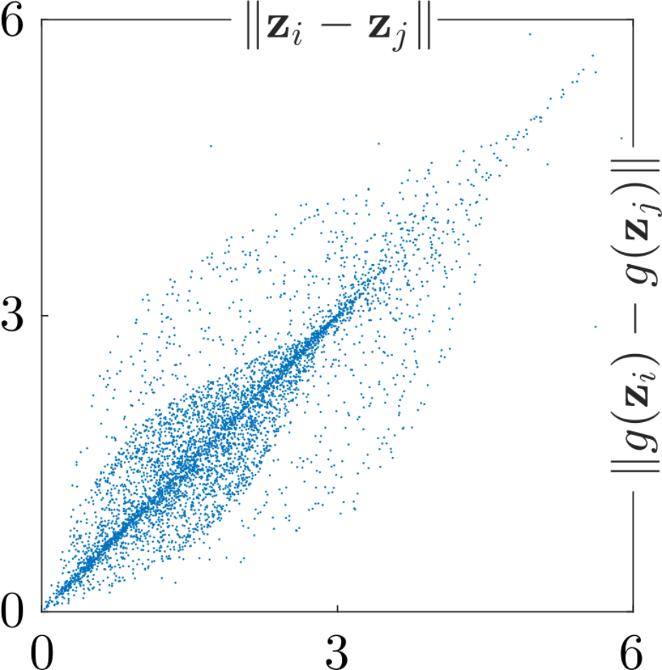
If we are to use the learned representation for becoming wiser about the underlying physical phenomena that generated the data, then clearly we cannot depend on the Euclidean assumption. Otherwise, whichever conclusion we arrive at will depend on whichever arbitrary parametrization we happen to recover. This is unsatisfactory!
What do we really want from a representation?
The main reason we keep treating the learned representation as being Euclidean is that we know how to engage with the representation. We know how to plot data, perform artihmetic, and more, when we have a Euclidean representation. Having these elementary tools available is convenient.
With this in mind, we might ask, what do we want from a representation? Put another way: which operations to we want to be able to perform in the new representation? The answer to such questions are inherently subjective, but some elementary operations might be easy to commonly agree upon. My subjective suggestions are
- Visualization: Being able to visually inspect data in the new representation is crucial for gaining intuitions about the underlying physical phenomena. We have develop tools for visualizing learned representations in a way that is invariant to reparametrizations.
- Distances: For quantitative evaluation we often need to determine which data points are similar, which imply some measure of such. Ideally, I'd like to see some metric distance measure that is invariant to reparametrizations. If we can go further and derive some associated notion of geodesic (shortest path between two points), then this is even more useful.
- Measure: If we are to build models in the new representation, having the ability to measure the probability of an event seems crucial. This in turn implies that we should be able to compute integrals over the learned representation.
- Arithmetic: Let's face it: plus and minus are nice tools to have. Being able to perform elementary arithmetic is something we take for granted all the time, and it's hard to let go of this ability. Consequently, it would be really nice to have basic operators akin to plus, minus, division, and multiplication available in this new representation.
It's not hard to come up with more operators that should be applicable in the learned representation. What's harder is finding a way to define such operators in a way that is invariant to reparametrizations to avoid arbitrariness...
Enough with the complaining; get to the solution!
In mathematics this type of problem is well-studied, and usually geometry provides a solution. The solution that we explore is to measure all we ever want to measure in the data space rather than in the new representation space. For example, to measure the length of a curve in latent space, we map all points along the curve into data space, and measure the length of the curve in this space. This approach gives rise to a Riemannian metric in the representation space, which put us on solid grounds mathematically.
In practice, a Riemannian interpretation of the representation is insufficient as we need to take the stochasticity of the generative process into account. This force us to develop new stochastic extensions to classic Riemannian geometry, and to develop the associated numerical tools in order to apply the theory in practice.
You can read more about this line of thinking in the papers below. If you want to talk more about this line of thinking, then do reach out (we’re nice people, and we’d love to chat with you!). Also: the team is expanding, so consider joining us :-)